Counting Cars with Raspberry Pi
In this post, I’ll walk you through a small part of my final project, where I run a convolutional neural network (CNN) on a Raspberry Pi 3 to detect cars in an image. While this might not be the most advanced method, it works surprisingly well, is fun to watch in action, and is very easy to set up by following the steps outlined here.
I’ll be using a convolutional neural network in combination with the YOLO (You Only Look Once) detection system.
Convolutional Neural Networks (CNNs)#
Commonly referred to by their acronym, CNNs are designed to efficiently process images. These networks mimic the brain’s behavior, specifically the neurons in the primary visual cortex, and use 2D matrices, which are highly effective for computer vision tasks.
In image analysis, CNNs perform two critical operations within their hidden layers, known as pooling and convolution.
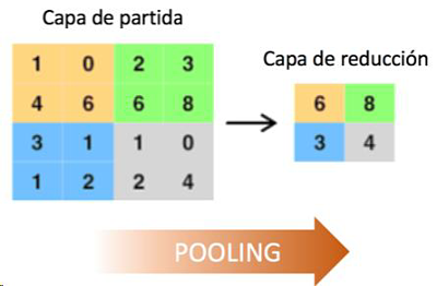
- Pooling: This operation reduces the size of the image, helping to decrease the computational load during processing.

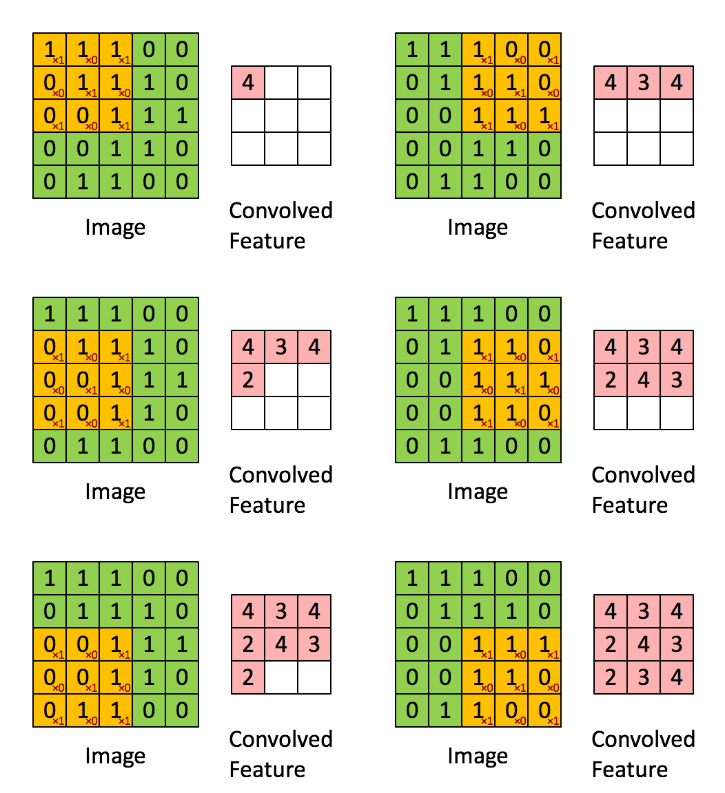
- Convolution: Convolutional layers use filters that move across the image, detecting important features while also reducing its size. This is done by performing multiplication and summation operations between the initial layer and the filter.

- Classification Layer: This layer operates like a traditional multilayer neural network, where each pixel is treated as a neuron. In simpler terms, if we start with a 10x10 image, we would have 100 neurons in this layer.
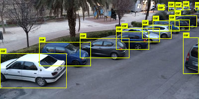
The final output looks like this:

YOLO#
YOLO is a powerful object detection algorithm that utilizes deep learning and convolutional neural networks. What sets YOLO apart is that, as the name suggests, it only requires a single pass through the image to make predictions, unlike other algorithms that need multiple passes. YOLO works by dividing the image into an SxS grid, where each cell predicts potential bounding boxes—rectangles indicating the location of detected objects. After making predictions, YOLO eliminates low-confidence bounding boxes.

Let’s Get to Work#
Requirements#
- Raspberry Pi 3 Model B+ (It also works with model B, but image quality may be compromised.)
- USB or CSI camera
- Basic Raspberry accessories such as: 5V power supply, microSD card with Raspbian installed, cases, etc.
I won’t go into detail about installing Raspbian or setting up basic Raspberry Pi software since there are countless tutorials available. The assumption here is that you already have a terminal set up on your board.
The first step is to install Git and download the repository for the neural network. This is a fork of the Darknet neural network.
sudo apt-get install git
git clone https://github.com/AlexeyAB/darknet
cd darknet
Once inside the repository, you’ll need to make some adjustments before compiling the code to ensure it runs smoothly on the Raspberry Pi. The Pi has a decent microprocessor, but if not properly configured, the neural network may throw a segmentation fault error due to limited memory.
sudo nano Makefile
Modify the following line:
- OPENMP=0 –> OPENMP=1
OpenMP provides concurrency for the neural network (written in C), allowing multiple processes to run simultaneously on the same core. This improves performance on the Pi’s microprocessor.
Next, adjust the settings in the configuration file:
sudo nano cfg/yolov3.cfg
If you are using a RaspberryPi3 Model B+, modify:
- width=608 –> width=416
- height=608 –> height=416
If you are using a RaspberryPi3 Model B, modify:
- width=608 –> width=224
- height=608 –> height=224
By doing this, we reduce the image size entering the neural network. Larger image sizes increase the computational load, so reducing the resolution is necessary, especially for the Model B.
Now, run the make command to compile the code.
make
This will generate the darknet executable. Once the neural network is compiled, you’ll need the pretrained weights:
wget https://pjreddie.com/media/files/yolov3.weights
Download the weights to the same directory where the darknet executable is located. That’s it! Each execution will take about two minutes. To run the object detection, use the detect command and provide the configuration file, pretrained model, and the image you want to analyze:
./darknet detect cfg/yolov3.cfg yolov3.weights data/prueba1.jpg
layer     filters    size              input                output
   0 conv     32  3 x 3 / 1   416 x 416 x   3   ->   416 x 416 x  32 0.299 BF
   1 conv     64  3 x 3 / 2   416 x 416 x  32   ->   208 x 208 x  64 1.595 BF
   2 conv     32  1 x 1 / 1   208 x 208 x  64   ->   208 x 208 x  32 0.177 BF
   3 conv     64  3 x 3 / 1   208 x 208 x  32   ->   208 x 208 x  64 1.595 BF
   4 Shortcut Layer: 1
   5 conv    128  3 x 3 / 2   208 x 208 x  64   ->   104 x 104 x 128 1.595 BF
   6 conv     64  1 x 1 / 1   104 x 104 x 128   ->   104 x 104 x  64 0.177 BF
   7 conv    128  3 x 3 / 1   104 x 104 x  64   ->   104 x 104 x 128 1.595 BF
   8 Shortcut Layer: 5
   9 conv     64  1 x 1 / 1   104 x 104 x 128   ->   104 x 104 x  64 0.177 BF
  10 conv    128  3 x 3 / 1   104 x 104 x  64   ->   104 x 104 x 128 1.595 BF
  ...
Results#
The output can be saved in a .txt file, which you can process to count the number of cars detected. Here’s how I did it:
./darknet detect cfg/yolov3.cfg yolov3.weights /home/pi/camera/cam.jpg > /home/pi/output_NN.txt
cat /home/pi/output_NN.txt | grep car | wc -l

I hope you found this guide interesting! Feel free to follow me on Twitter if you’d like to keep up with my work.
Bye!